Examples

Eighteen examples come with MaveScape. Three are published experiments from MaveDB, their counts unchanged and bundled: two populations, a growth time series and sorted bins. Five are opened from MaveDB when you open them: published scores alone, with their record; a saturation genome editing screen of nucleotide variants on a RefSeq transcript, with its counts; two score sets of one enzyme opened together as two conditions; a score set rescored from its counts, deposited and opened again; and two laboratories' screens of one protein, compared on one scale. Three calibrate published scores of BRCA1, TP53 and PTEN against ClinVar's records of the gene, which they bring. Seven are simulated, with every true effect known: two populations, a time series, a sort, a barcoded library, two conditions from shared inputs, an experiment with two problems planted, and a calibration whose labels are half made from the assay itself. Each opens scored, with its question, guided steps of a few minutes and what to expect, in the inspector.

GRB2 SH3 domain (published)

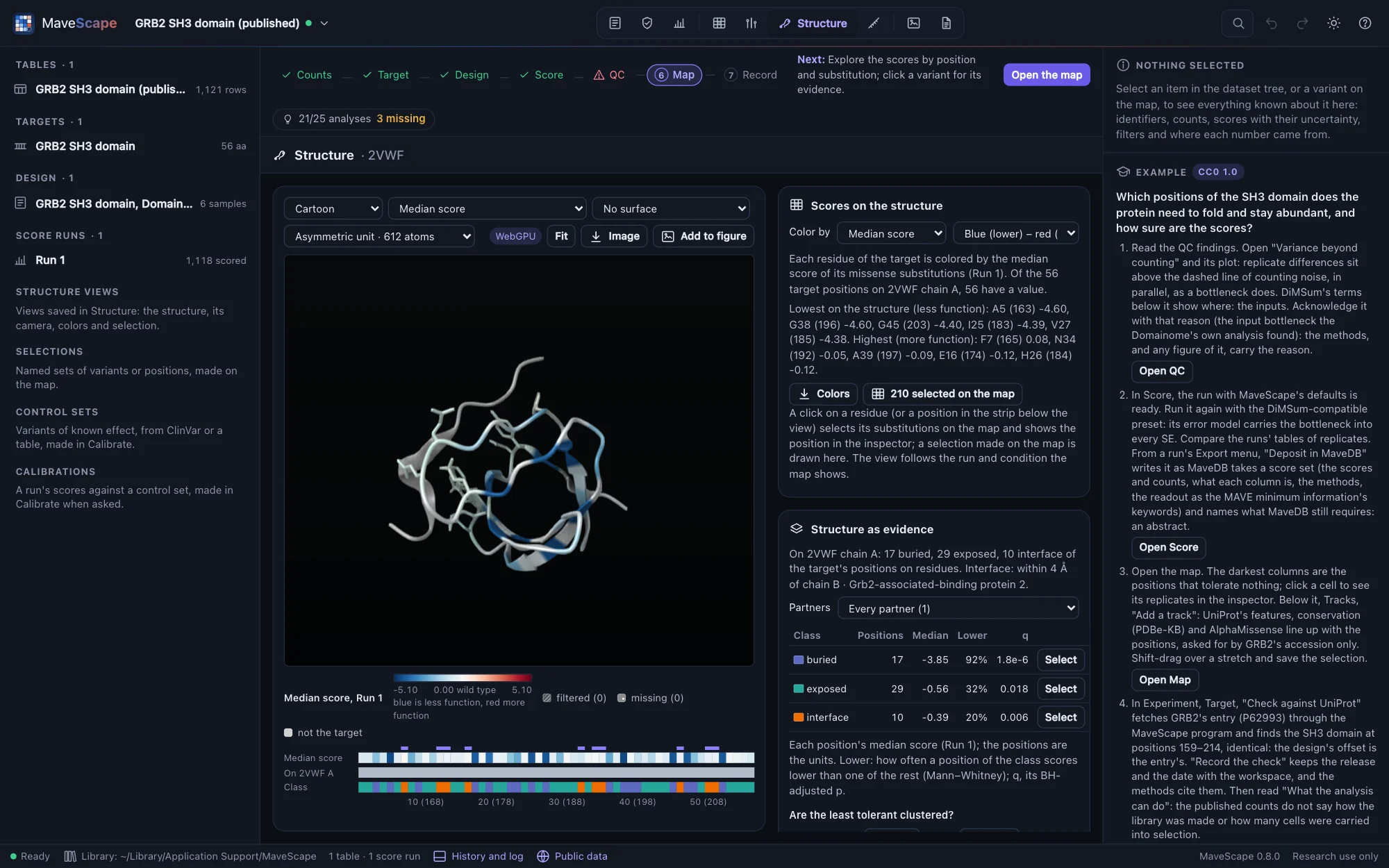
An abundance selection of every substitution in the 56-residue SH3 domain of GRB2, in three replicates, from the Human Domainome (MaveDB urn:mavedb:00000835-a-1, CC0 1.0; Beltran et al., Nature 2025). The counts are MaveDB's file, unchanged.

The question: which positions does the domain need to fold and stay abundant, and how sure are the scores?

The QC view of the GRB2 example with the variance beyond counting failing at 11.4 times the counting variance — What to expect in QC: everything passes but the variance beyond counting, about 11×.

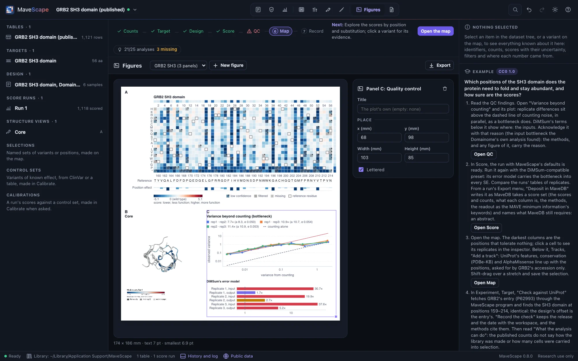
Quality control passes everything except the variance beyond counting, about 11×: a bottleneck. DiMSum's error model puts it at the input, 20 to 38 times counting, as the Domainome's own analysis found; scored with the DiMSum-compatible preset, every SE carries it.
Nonsense variants score about −4.6 against the wild type's 0: the assay separates loss of function cleanly.
The least tolerant positions are buried hydrophobic and glycine residues of the fold: A163, G196, G203 and I183 on GRB2's numbering.
In Experiment, What the analysis can do: 19 of 25 analyses are ready. The published counts do not say how the library was made or how many cells were carried into selection; with the cells, QC would check the bottleneck it finds against them. The library is protein-level, so there are no synonymous variants to normalize to.
In Compare, against its record's published scores (kept beside the workspace without opening it), Run 1 agrees at r 0.997 on another scale; rescaled by their anchors, Lin's concordance is 0.996 and the bias 0.009. Against AlphaMissense, ρ 0.55 by rank, and an AUC of 0.78 between its classes.
In Structure, on 2VWF (the SH3 domain holding a peptide of Gab2) colored by each position's median score, the least tolerant residues pack the core: the ten lowest have a median of 20.5 Cα atoms within 10 Å, the ten highest 14.5. The ten residues that touch the peptide are tolerant (a median of −0.39, against −0.81 for the rest): the assay measured abundance, not binding. Click I183, and its 19 substitutions are selected on the map and the position is in the inspector. Save the view as Core under Saved views: it reopens as it is with the workspace, and goes into its archive and methods.

GRB2's SH3 domain on 2VWF colored by the median score, the core dark blue, the residues that touch the Gab2 peptide pale and drawn as sticks — GRB2's SH3 domain on 2VWF, colored by the median score: the core dark blue, the peptide's neighbors (sticks) pale.

The guide ends with a figure of what it found: Run 1's map, the view Core and the variance beyond counting on one page, the finding acknowledged in QC with its reason (the input bottleneck the Domainome's own analysis found). Exported as PDF, the figure carries its manifest: Run 1 by its output's SHA-256, the QC thresholds and the acknowledgement's reason, 2VWF and the view's image by theirs. Dropped on the window, each panel is as it was drawn; once the table is scored again, the map and the QC panel say so.

The Figures view with GRB2's figure on a page two columns wide: A, Run 1's map with the sequence and the position effect below it; B, 2VWF colored by the median score; C, the variance beyond counting, the replicate differences above the dashed line of counting and DiMSum's terms of each input and output; panel C selected, its properties beside the page — GRB2's figure: the scores, where the least tolerant residues sit, and the bottleneck behind every SE.

Hsp90 over 21 generations (published)

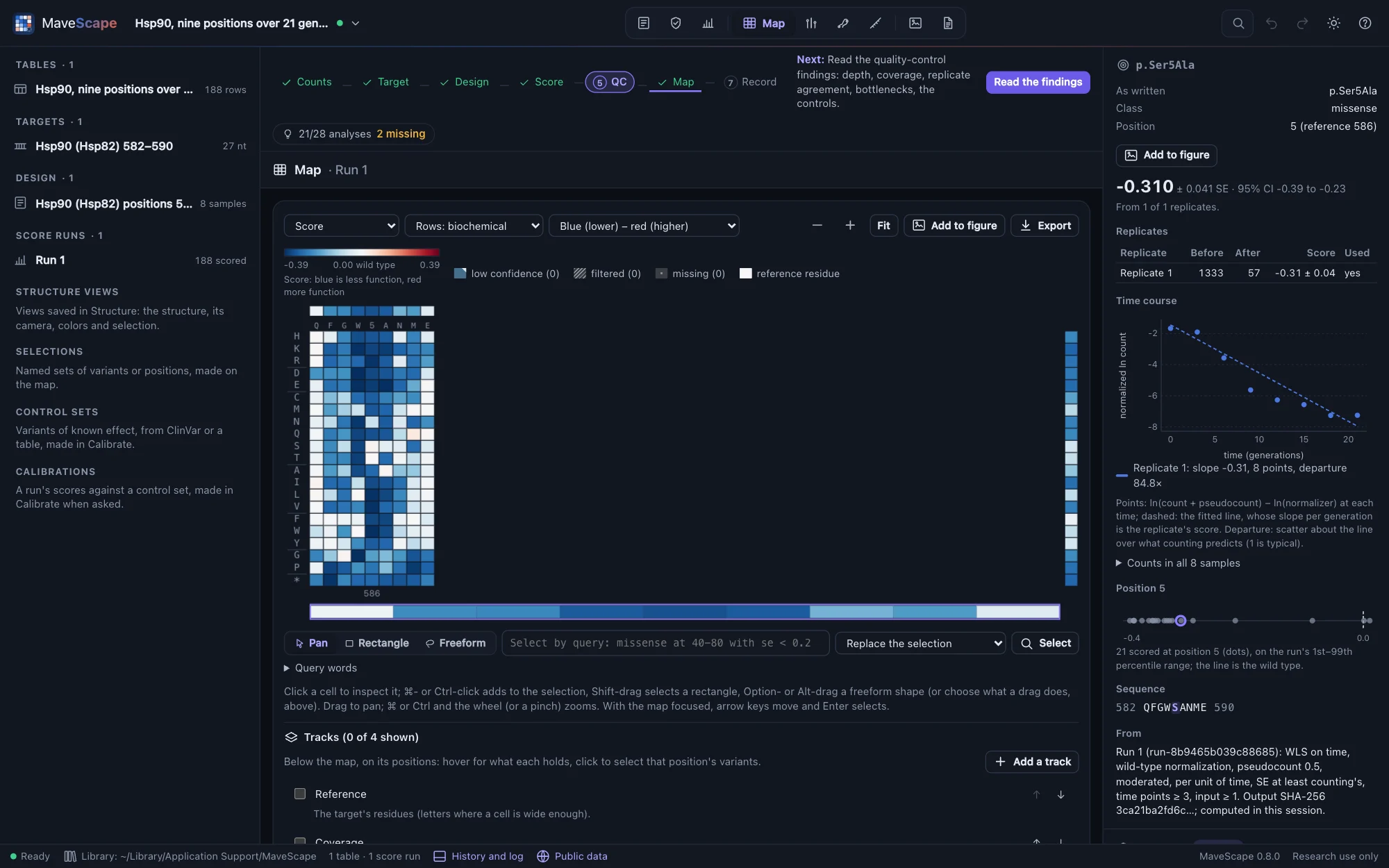
Every codon at nine positions (582–590) of yeast Hsp90 (Hsp82), selected by growth with the cells' own Hsp90 inactivated and sampled eight times over 21 generations, in one replicate: the first EMPIRIC experiment (MaveDB urn:mavedb:00000011-a-1, CC0 1.0; Hietpas, Jensen and Bolon, PNAS 2011). The counts are MaveDB's file, unchanged.

The question: how fast does each variant grow per generation, which of the nine positions tolerate change, and what can one replicate tell and not tell?

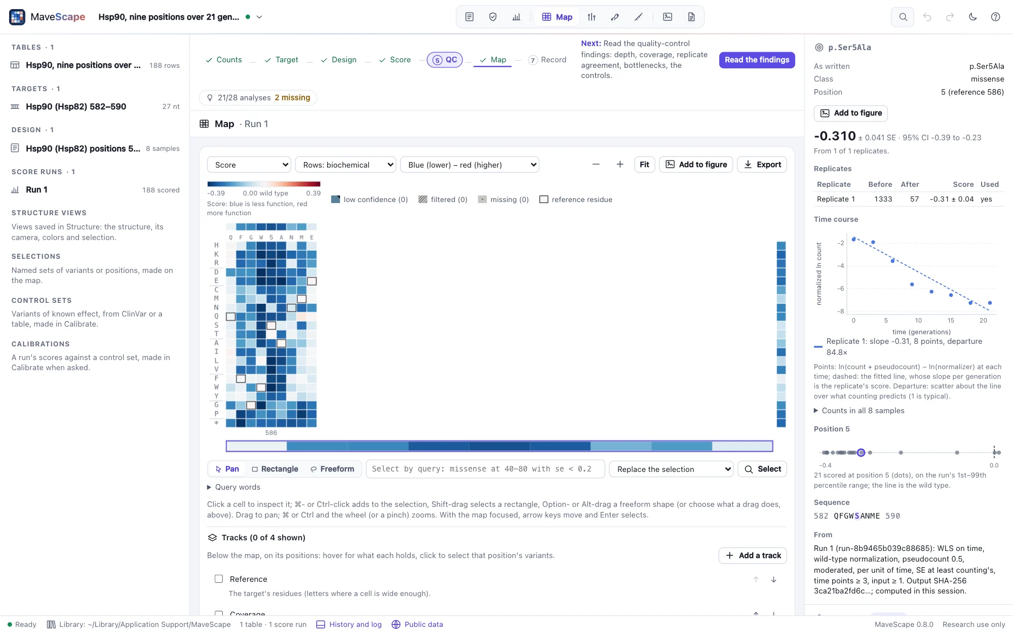
The map of the Hsp90 example: nine positions by every substitution, positions 585 to 587 darkest; the inspector shows p.Ser5Ala at reference position 586 scoring −0.31 per generation, with its time course falling over 21 generations — Hsp90 per generation: positions 585–587 tolerate almost nothing. The inspector draws a variant's time course in its one replicate.

MaveDB names each codon variant on its own row, and writes the wild type once per position. Read as codon variants, the 568 rows become 188 protein variants: each substitution's codons combined, the wild type's nine identical copies read once.
The example scores per generation (the times are generations). Positions 585–587 (W, S, A) tolerate almost nothing, 582 and 590 almost everything; synonymous codons score near 0.
Where the authors fit every time point, the scores follow the published fitness with r 0.95, a median 0.005 per generation apart. The record says its slopes are of log₂ ratios, but they are of natural logarithms, as MaveScape's are. Stops score about −0.32 against the published −0.77: the authors fit null-like variants on their first three time points, before they reach the floor.
Quality control fails the fit of the time courses, about 44× what counting predicts, so each slope's SE comes from its own residuals. With one replicate, nothing between replicates is assessed: What the analysis can do says so, and that the record gives no MaveDB terms for the assay or the library.
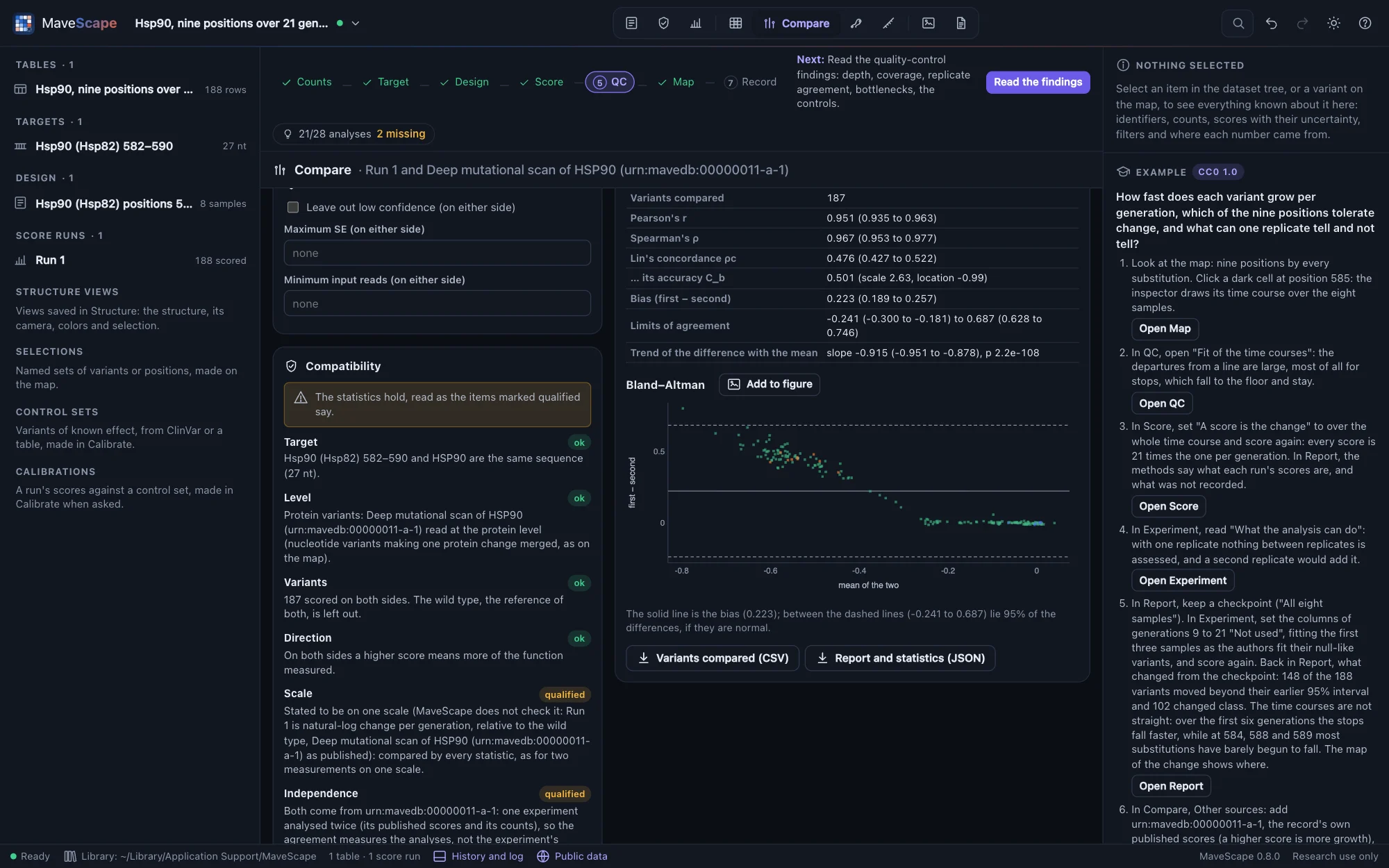
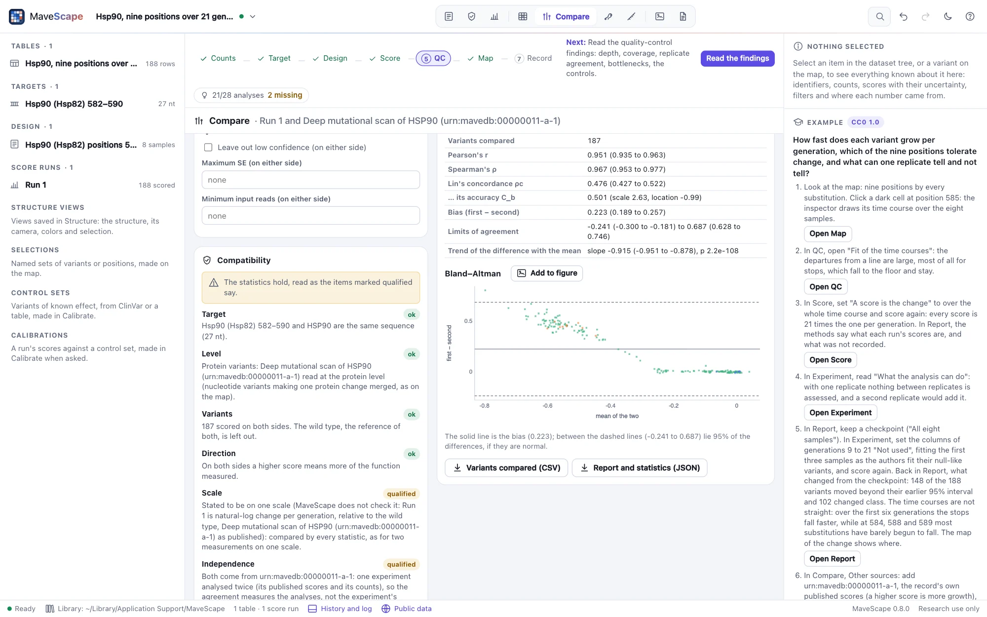
A rescoring against the published scores (Comparisons): the record's own scores, kept beside the workspace, correlate with Run 1 at r 0.95, but stated to be on one scale their Lin's concordance is only 0.48, with a bias of 0.22. The difference grows with the effect (a Bland–Altman slope of −0.91), most at 585–587: how deleterious the null-like variants are depends on the time points fitted, a choice the authors made otherwise.
That choice, tried: in the Report view, a checkpoint before the first three samples are fitted (generations 9 to 21 set "Not used" in Experiment), as the authors fit their null-like variants. 148 of the 188 variants move beyond their earlier 95% interval and 102 change class, 93 from lower than the wild type to like it. The time courses bend: the stops fall faster at first (a median of −0.41 per generation over six generations, −0.32 over 21, still not the published −0.77), while at 584, 588 and 589 most substitutions have barely begun to fall (medians of about −0.02 per generation, against −0.16 to −0.26). The pseudocount, by contrast, moves none (0.5 → 0.1): weighted regression gives the few reads at the floor little weight.

The Compare view of Hsp90's Run 1 against its record's published scores, stated to be on one scale: 187 variants, Pearson's r 0.951, Lin's concordance 0.476, a bias of 0.223, and the Bland–Altman plot whose differences rise as the mean falls — Hsp90's Run 1 against its record's published scores: correlated, but not in agreement. The differences grow with the effect.

The Report view with the changes since the checkpoint All eight samples: the design's samples of generations 9 to 21 removed and their columns set aside, Run 3 scored; Run 2 to Run 3, 148 of 188 variants moved beyond their earlier 95% interval in Run 2's units and 102 changed class; the variants that moved most and the map of the change — What fitting the first three samples moves: most variants, in both directions.

Coagulation factor IX in sorted bins (published)

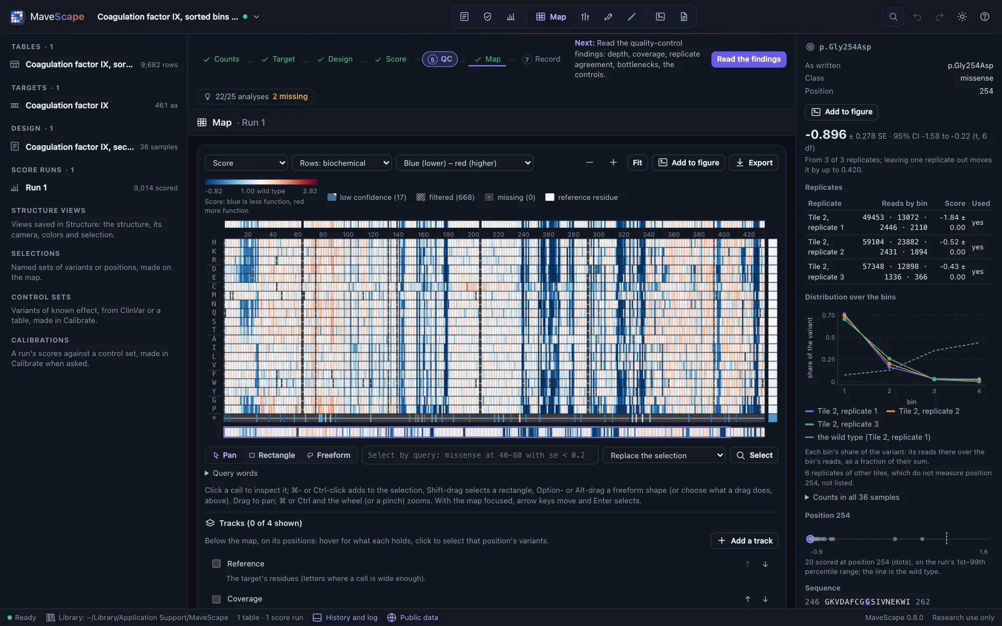
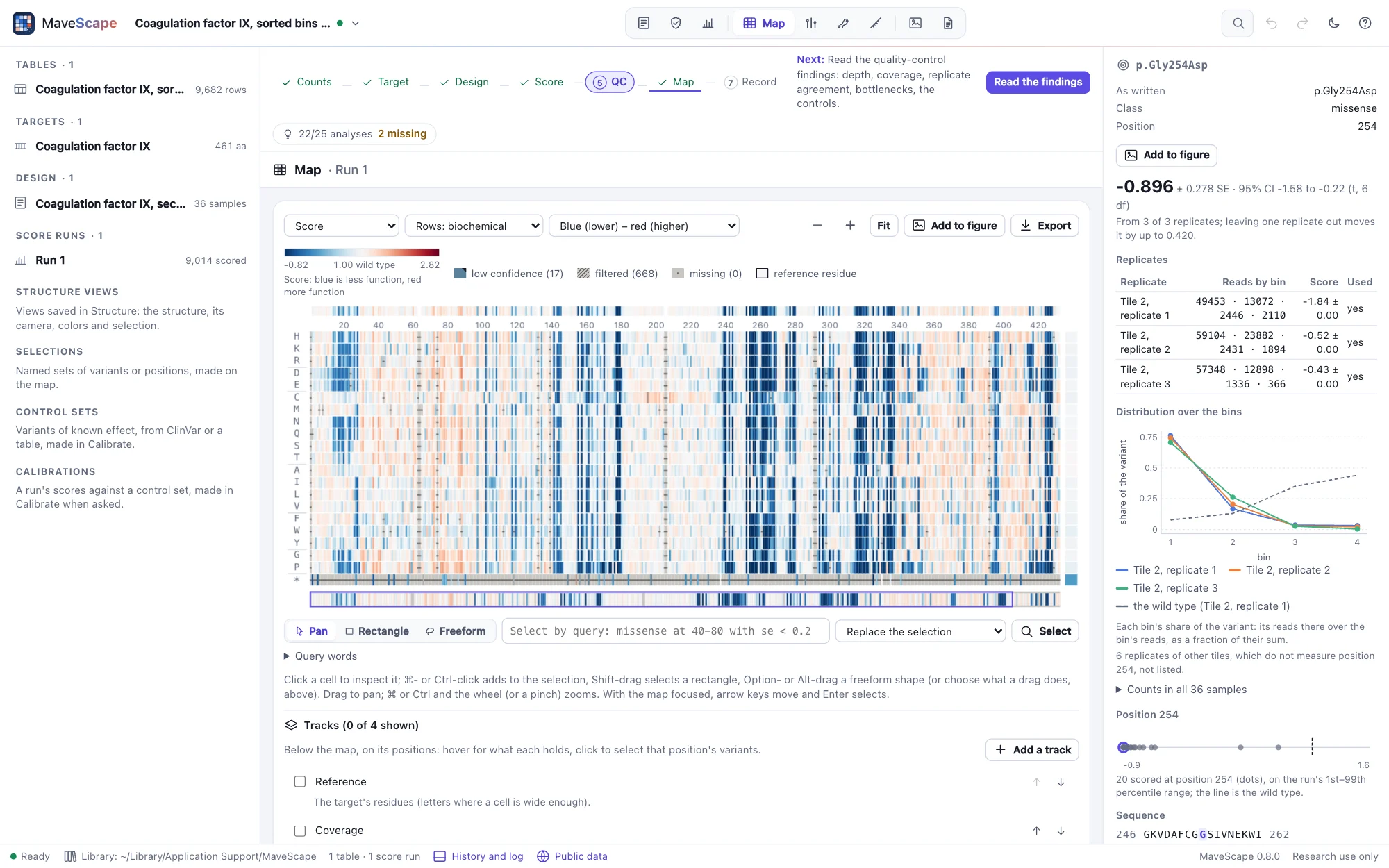
Every substitution of the 461-residue factor IX, secreted from human cells and displayed on their surface (MultiSTEP), stained at its C-terminal strep II tag and sorted into four bins, in three overlapping tiles of three replicates (MaveDB urn:mavedb:00001200-a-1, CC0 1.0; Popp et al., Nature Structural & Molecular Biology 2025). The counts are MaveDB's file, unchanged.

The question: which factor IX variants are still secreted, and how sure are the scores when the reads far outnumber the cells sorted?

The map of the factor IX example over 461 positions, the protease domain's dark columns; the inspector shows p.Gly254Asp measured in tile 2's three replicates, scoring −0.90, and its distribution over the four bins beside the wild type's — Factor IX: the protease domain holds most of the positions that tolerate nothing. A variant's distribution over the bins, beside the wild type's.

Positions 146–164 and 299–318 are measured in two tiles; their scores combine both.
Quality control fails the variance beyond counting, about 2,300×: some 10,000 reads per variant in each bin far exceed the cells sorted. The moderated combination carries the excess into every SE.
The cells per bin are not assessed, and the bins cannot be scored by maximum likelihood: MaveDB records neither the cells sorted nor the gates, which the sorter's report has.
With MaveScape's defaults (each replicate scaled to nonsense 0 and wild type 1) the scores follow the published ones with r 0.994. With MultiSTEP's own scale (the lowest 5% of missense at 0) and the replicates' mean, set in the Score view, r 0.9995; on that scale the nonsense median is 0.47.
With UniProt's features beside the map, the query missense from C in feature disulfide selects the substitutions of the 22 cysteines in factor IX's 11 disulfide bonds: 345 of the 399 scored are lower than the wild type beyond their uncertainty, against 2,124 of the 8,529 missense variants scored in all. Saved as a selection, missense and lower and not in Disulfides selects the rest (Selections).
In the Structure view, the PDB entry 1RFN (activated factor IX, X-ray at 2.8 Å) holds the protease domain (chain A) and the second EGF domain (chain B): 14 of the cysteines, in seven of the disulfide bonds, one of them joining the two chains. resn CYS selects them, drawn as sticks. Mapped onto it, the target is on chain A at 227–461, all identical, though the entry numbers it as chymotrypsin is numbered, and on chain B at 132–188, where SIFTS places it too; the entry's own record numbers chain B five earlier (Structures).

PTEN abundance, opened from MaveDB (published scores)

VAMP-seq abundance of 4,409 PTEN variants, as MaveDB publishes them (urn:mavedb:00000013-a-1, CC0 1.0; Matreyek et al., Nature Genetics 2018): scores alone, scaled with the wild type at 1 and nonsense at 0, with their standard errors and 95% intervals, and no counts. Opened from MaveDB through MaveScape's list of public services when you open it (1.7 MB, then cached), its table checked against the checksum it had when the example was made. It needs the MaveScape program.

The question: what can a published record of scores alone show, what does it leave out, and where would the rest be found?

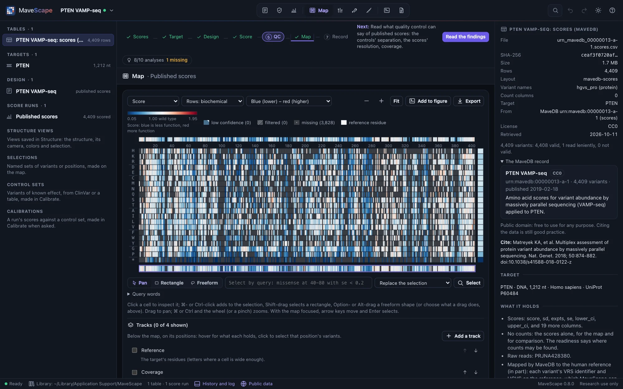
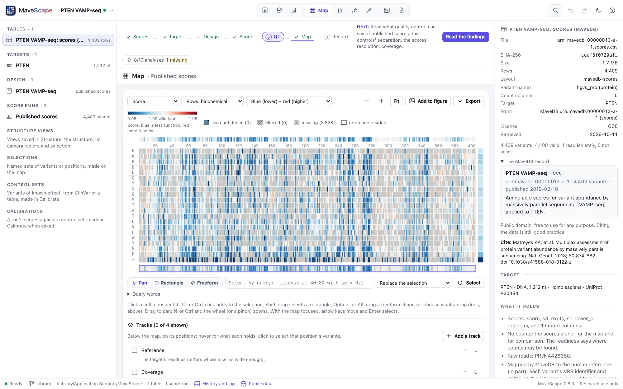
The map of PTEN's published abundance scores over 404 positions, the wild type at 1.00; the inspector shows the scores table opened from MaveDB, CC0, retrieved 2026-10-11, and the record: PTEN VAMP-seq, its citation, target and what it holds — PTEN's abundance as MaveDB publishes it, and the record in the inspector.

All 4,409 variants have a score, read as published: synonymous median 1.00, nonsense 0.06, the controls well separated (AUC 0.98).
About a quarter of missense variants score below 0.5; the least tolerant positions are spread through both the phosphatase and the C2 domain, as a stability readout expects.
The record gives the assay in MaveDB's terms (a reporter, loss of function, human cells, a library by oligo-directed mutagenic PCR), which become the design's readout, but not what a higher score means: the example states it from the paper. Its six calibrations are in the inspector, ExCALIBR's for research use only.
QC passes what it can assess from scores alone but coverage, 53% of all substitutions. Rescoring and QC of the counts need counts, which MaveDB does not hold for this record: the readiness says where they may be (the paper's supplement, the authors' repository, the raw reads PRJNA428380).
In Compare, against PTEN's lipid phosphatase activity (urn:mavedb:00000054-a-1, Mighell et al. 2018, kept beside the workspace without opening it), abundance agrees only in part (4,057 variants, r 0.45, ρ 0.37): two assays, and a variant can be stable but inactive. Rescaled by their anchors, the report shows the activity record's wild type is its row, 1 with an SE of 0, though its methods place wild type-like variants from −1.11 to 0.89. Against AlphaMissense, abundance tells its likely benign substitutions from its likely pathogenic ones with an AUC of 0.77.
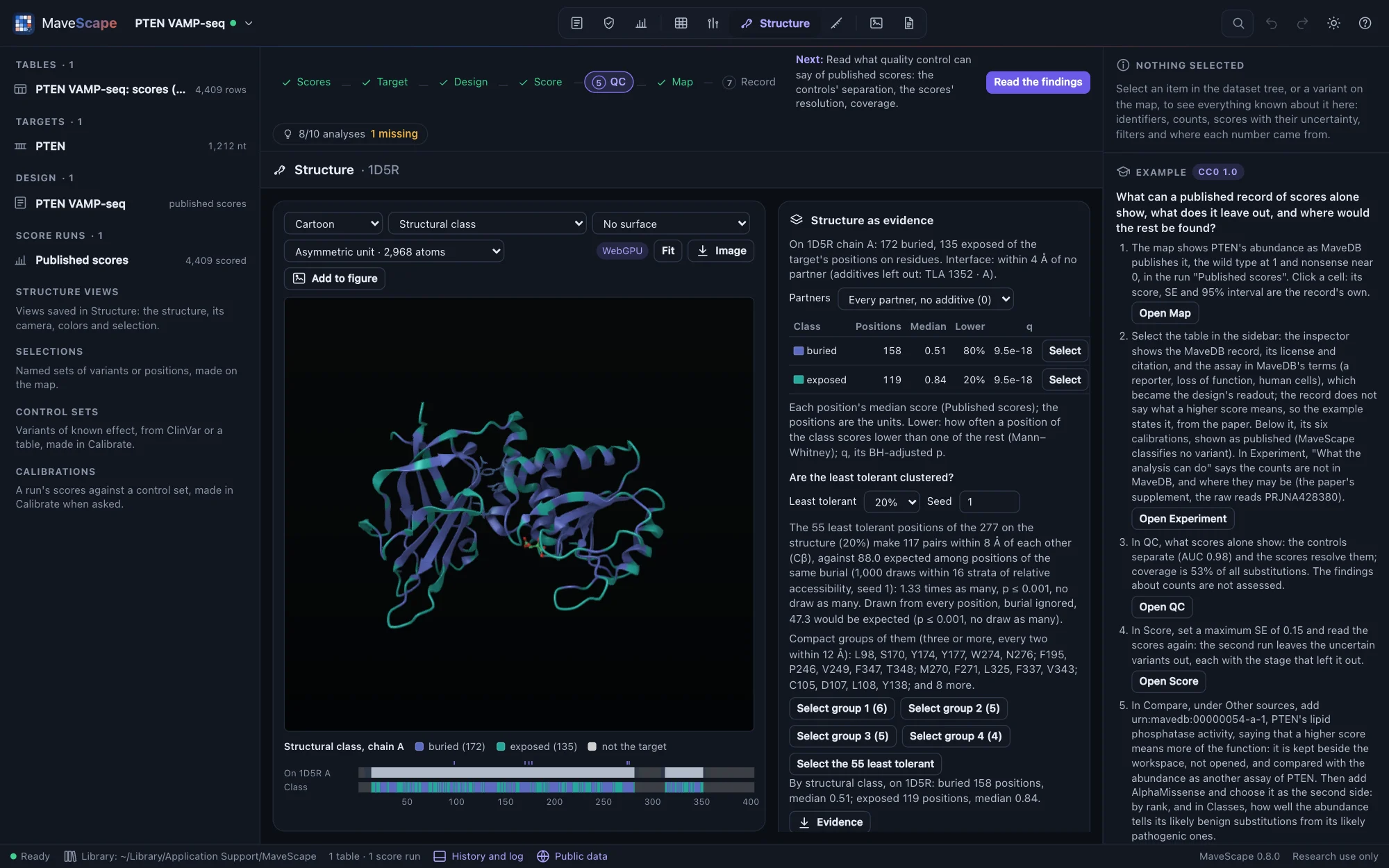
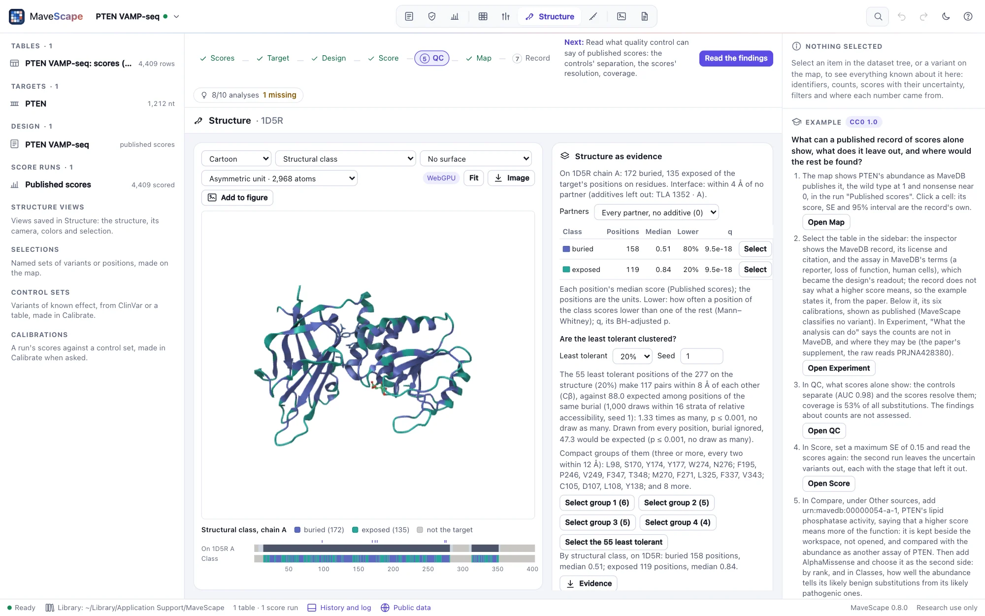
In Structure, on 1D5R (PTEN's phosphatase and C2 domains), buried positions (158) score a median of 0.51, exposed ones (119) 0.84: a buried position scores lower 80% of the time, as an abundance assay expects. The 55 least tolerant positions make 117 pairs within 8 Å, against 88.0 among positions as buried and 47.3 among any: beyond their burial they cluster, one compact group joining the two domains (L98, S170, Y174, Y177 with W274 and N276).

PTEN on 1D5R colored by structural class, with the pane Structure as evidence — PTEN on 1D5R by structural class, and the scores read by class.

BRCA1 saturation genome editing, opened from MaveDB (nucleotide variants)

3,893 single-nucleotide variants of 13 exons of BRCA1 and their flanking introns, edited into the genome of HAP1 cells, which need BRCA1 to grow (urn:mavedb:00000097-0-2, CC0 1.0; Findlay et al., Nature 2018): named on the RefSeq transcript NM_007294.3, scored by their depletion between day 5 and day 11, with the counts the authors deposited. Opened from MaveDB when you open it (1 MB, then cached), its tables checked against their checksums, and its transcript fetched from NCBI. It needs the MaveScape program.

The question: what do nucleotide variants of a gene do to its protein, which of them can a map of substitutions not show, and how close do the deposited counts come to the published scores?

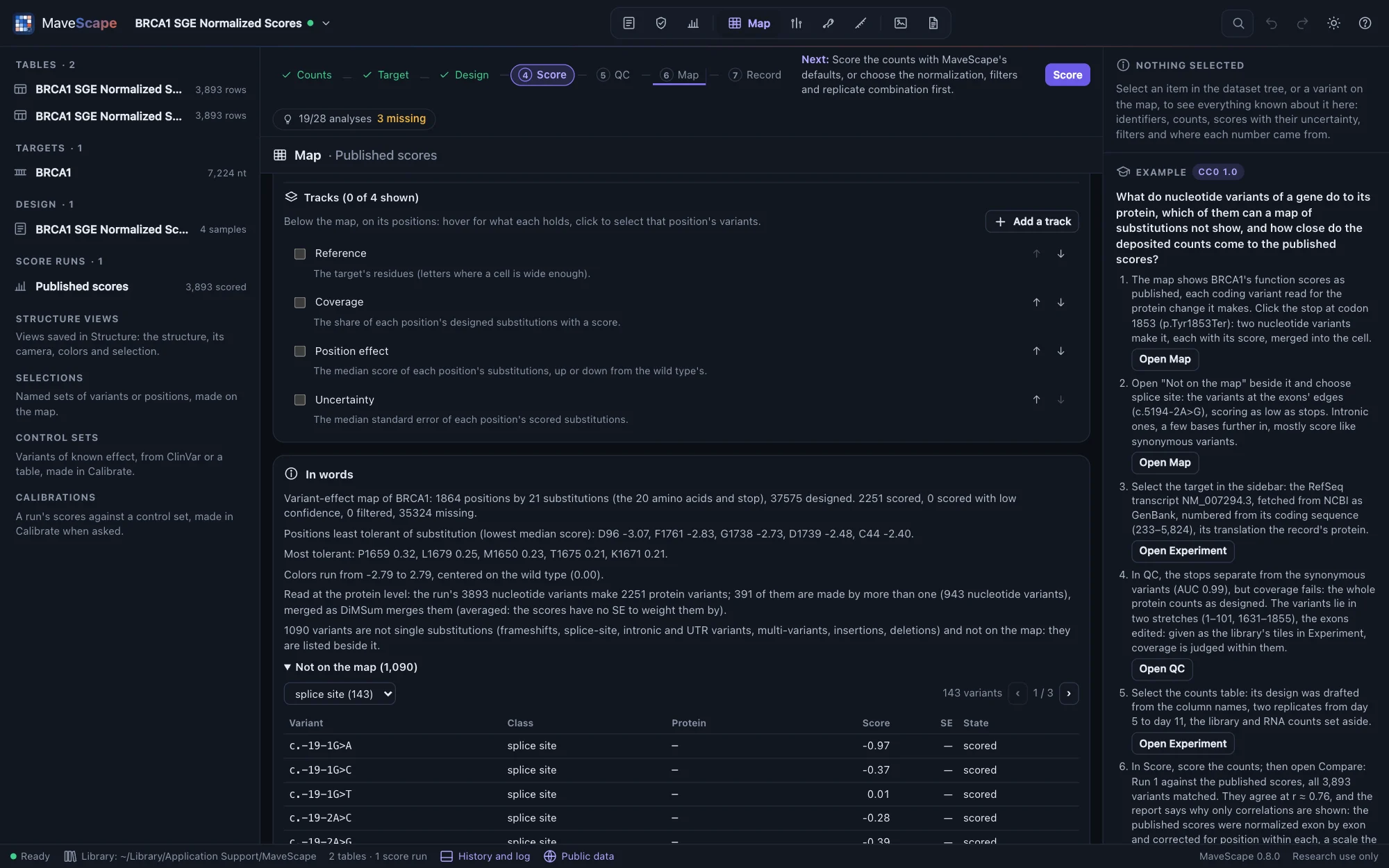
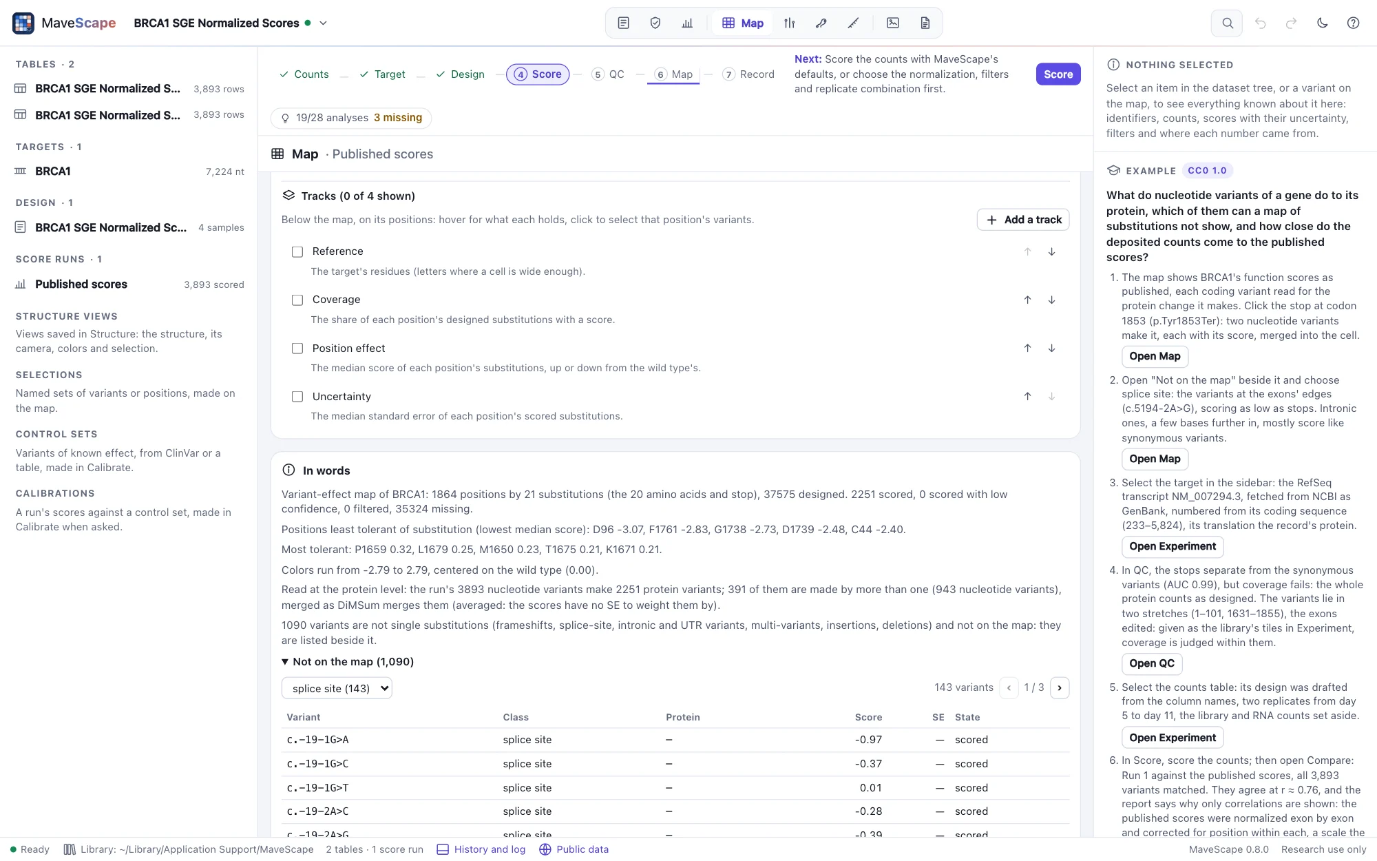
The map of BRCA1's saturation genome editing scores at the protein level, two stretches of the protein scored; in words, the 3,893 nucleotide variants make 2,251 protein variants; below, Not on the map — BRCA1's function scores at the protein level, and the splice-site variants beside the map.

Every one of the 3,893 variants is valid on NM_007294.3: 2,077 missense, 579 synonymous, 138 nonsense and 9 at the start codon, with 891 intronic, 143 at splice sites and 56 in the 5′ UTR.
On the map, the coding variants read at the protein level: 2,251 protein variants, 391 made by more than one nucleotide variant and merged. The 1,090 with no protein change to draw are listed beside the map.
Nonsense variants score far below synonymous ones (medians −2.12 and −0.01; AUC 0.99). Splice-site variants score like nonsense (median −2.02); intronic ones a few bases further in, like synonymous ones (median −0.18).
QC fails coverage: 17% of the substitutions one base change makes, on the whole protein. The variants lie in two stretches, positions 1–101 and 1631–1855: the exons the experiment edited. Given as the library's tiles, coverage is judged within them.
The counts open with a design drafted from their names: two replicates, day 5 to day 11, the library and RNA counts set aside. Scored, they agree with the published scores at r ≈ 0.76 in the Compare view, which gives correlations only and says why: the authors normalized each exon apart and corrected for position within it, a scale the counts do not record (Comparisons).

DHFR with and without the Lon protease, opened from MaveDB (two conditions)

Every substitution of E. coli's dihydrofolate reductase (DHFR, 159 residues), on a plasmid in a strain without its own DHFR, grown in a turbidostat and sampled at 0, 2, 4, 6, 8, 12, 16 and 18 hours (Thompson et al., eLife 2020). The strain lacks the Lon protease, as all B strains do (−Lon, urn:mavedb:00000063-b-1); the experiment was repeated with Lon restored (+Lon, urn:mavedb:00000063-a-1). MaveDB keeps the two as score sets of their own, CC0 1.0. The example opens both together (2.4 MB, then cached), each table checked against the checksum it had when the example was made, and joins their counts into one experiment of two conditions. It needs the MaveScape program.

The question: which substitutions does Lon penalize, how sure is each difference, and where in the protein are they?

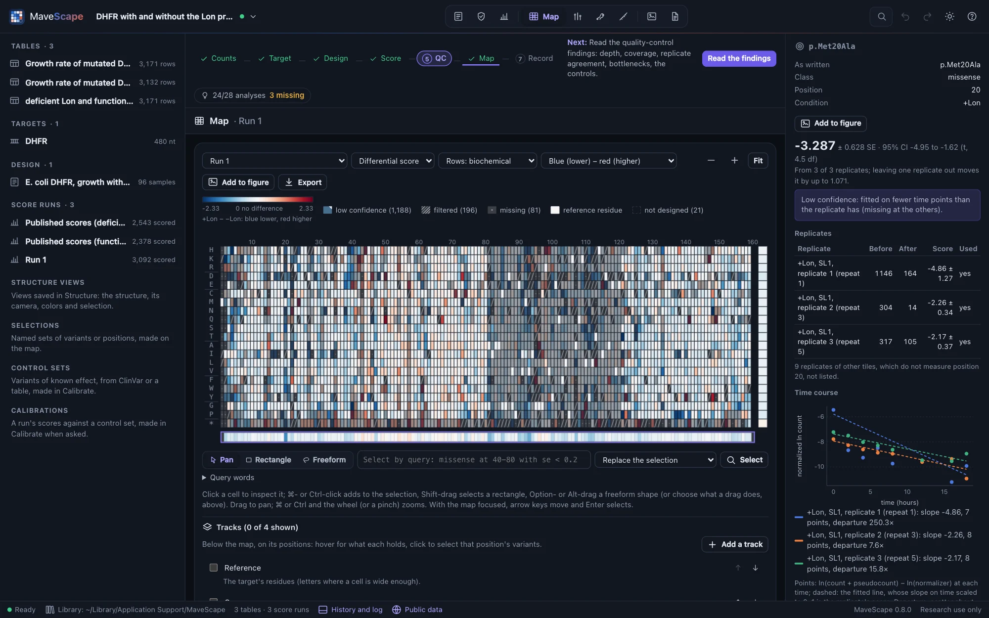
The map of DHFR colored by the difference +Lon minus −Lon over 160 positions, mostly blue; the inspector shows p.Met20Ala in +Lon scoring −3.29 from the three replicates of sub-library SL1, nine replicates of other tiles not listed, and their time courses over 18 hours — The map of +Lon − −Lon: Lon penalizes most of the substitutions it touches. The inspector lists only the variant's own sub-library's replicates.

The design is the paper's: four sub-libraries of 40 positions, each grown three times, two in each of the six repeats per condition, paired differently in each condition. Each repeat's samples hold two sub-libraries, and each replicate measures only its own tile's positions: no measurement is combined twice. The transformation and outgrowth samples are set aside.
With MaveScape's defaults (weighted regression) the scores follow the published ones at r ≈ 0.90 without Lon and 0.96 with it. With the authors' unweighted regression (ordinary least squares), r ≈ 0.96 and 0.98, on the same scale: the published scores are Enrich2's slopes over the whole 18 hours.
Without Lon about twice as many substitutions grow faster than the wild type (a score above 0.2) as with it: 877 and 391 here, 736 and 384 published. The difference is negative for 92% of the 376 substitutions it calls at q < 0.05, and most negative at native hydrophobic residues (a mean of −0.48 per position, against −0.20 elsewhere), as the paper found for the buried core. The conditions share no input (each strain was transformed apart), so they are compared as independent.
QC fails the variance beyond counting and the fit of the time courses, and reviews the time points used and the dropout: a variant below 2 × 10⁻⁵ of the reads was not reported at a time point, so the most depleted drop out and their slopes rest on the early time points, as the authors' did.

BRCA1 RING domain, from MaveDB and back (round trip)

E3 ubiquitin ligase activity of 12,316 amino-acid variants of the BRCA1 RING domain (codons 2–304), displayed on phage and selected over five rounds for their own ubiquitination, in two library preparations of three replicates (Starita et al., Genetics 2015; scored by Enrich2, Rubin et al., Genome Biology 2017; urn:mavedb:00000003-a-2, CC0 1.0). Opened from MaveDB with its counts (7.8 MB, then cached) and the design the record's method text and the paper describe, which the counts' names do not: their table holds the yeast two-hybrid assay too, a separate experiment. It needs the MaveScape program.

The question: does rescoring the counts reproduce the published scores, and does a deposit carry the scores and their record back to MaveDB without loss?

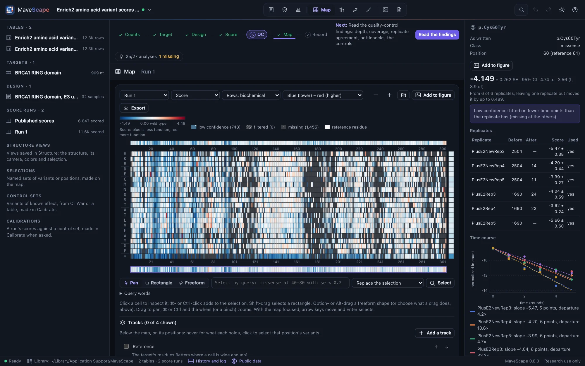
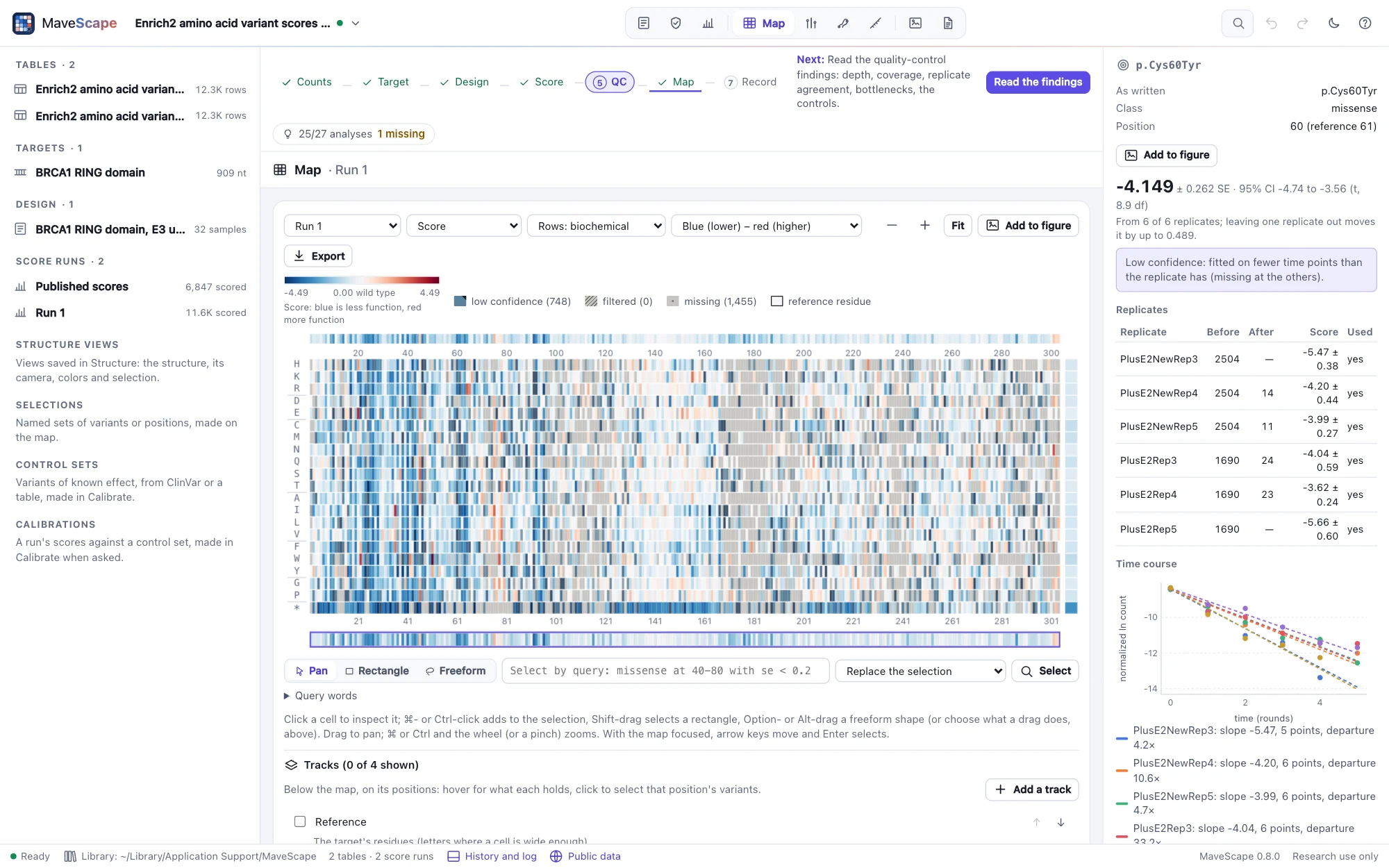
The map of the BRCA1 RING domain scored from its counts, 303 positions; the inspector shows p.Cys60Tyr, BRCA1 residue 61, a zinc ligand, scoring −4.15 from six replicates, each falling over the rounds — Run 1 on the map; a zinc ligand of the RING in the inspector, its six replicates.

With MaveScape's defaults every replicate score equals the published one (50,055 of them, within 2 × 10⁻¹⁴): weighted regression with wild-type normalization is Enrich2's. The combined scores differ a little (r 0.992): MaveScape's moderated combination against Enrich2's random effects. With the Enrich2-compatible preset they follow the published ones (r 1.000), 6,847 scored, as many as MaveDB's.
The RING's eight zinc ligands (C24, C27, C39, H41, C44, C47, C61 and C64 on BRCA1's numbering) are among its twelve least tolerant positions, their median scores about −3 against −0.7 for a typical position.
From Run 1's Export menu, Deposit in MaveDB writes the run as MaveDB takes a score set, its experiment described as the record's (give urn:mavedb:00000003-a to add the score set to it). Dropped on the window, the package opens as a record does: its scores, read as published, are Run 1's exactly, and written again it is the same bytes.
QC fails the variance beyond counting and the fit of the time courses: over five rounds most variants that lose activity fall below detection, as stops do.
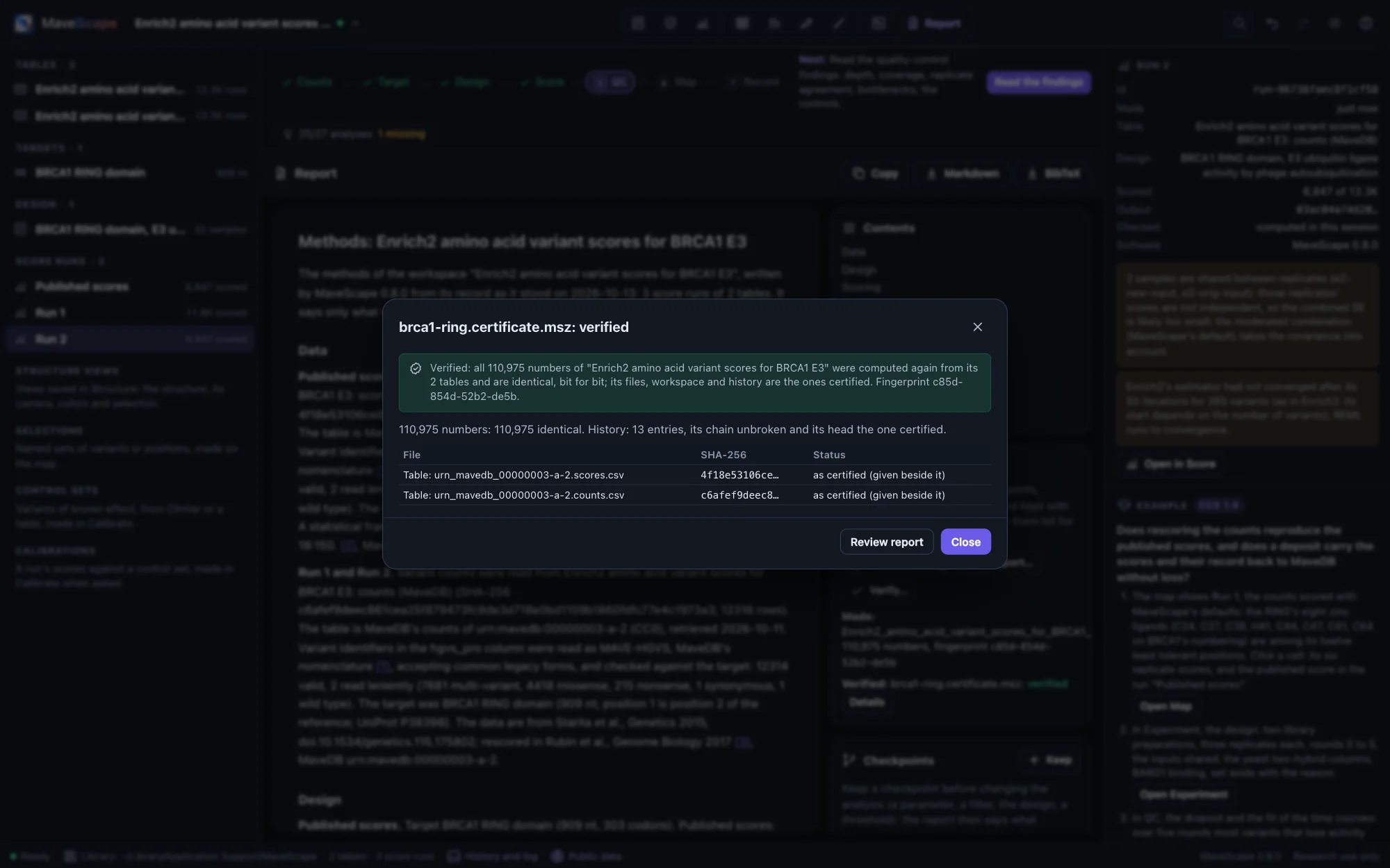
Certified with the published scores, Run 1 and the Enrich2 rescoring, its 110,975 numbers are computed again from MaveDB's two tables and verified bit for bit; the review report holds them in one file. Certified without its tables, the certificate names them by the SHA-256 of MaveDB's files (the scores 4f18e531…, the counts c6afef9d…): alone it is not checkable, and with the two files downloaded from the record (mavescape verify --data) it is verified.

The Report view with the verification of BRCA1 RING's certificate made without its tables: all 110,975 numbers computed again from MaveDB's two tables, given beside it, and identical, bit for bit; the two tables listed as supplied; the Certificate pane beside the report — BRCA1 RING's certificate, made without its tables, verified with MaveDB's two files beside it.

TP53, two screens on two scales, opened from MaveDB (published scores)

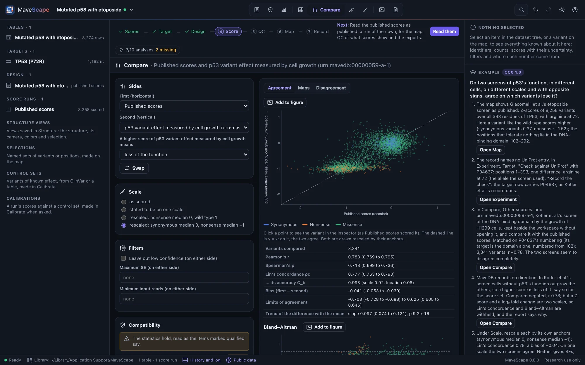
Every substitution of full-length TP53, with arginine at 72, expressed in p53-null A549 cells under etoposide and scored as Z-scores (Giacomelli et al., Nature Genetics 2018; urn:mavedb:00000068-c-1, CC0 1.0), and an independent screen of its DNA-binding domain by the growth of H1299 cells, scored as log₂ fold changes (Kotler et al., Molecular Cell 2018; urn:mavedb:00000059-a-1, CC0 1.0), with Giacomelli et al.'s nutlin-3 screen of the same library (urn:mavedb:00000068-b-1). The first is opened (its published scores; MaveDB has no counts for it); the others are kept beside the workspace and compared without opening them. It needs the MaveScape program.

The question: do two screens of p53's function, in different cells, on different scales and with opposite signs, agree on which variants lose it?

The Compare view of the TP53 example: the etoposide screen's published scores against Kotler et al.'s screen of the DNA-binding domain, both rescaled by their synonymous and nonsense medians: 3,341 variants, Pearson's r 0.783, Lin's concordance 0.777, a bias of −0.041; the scatter plot along the line y = x — The etoposide screen against Kotler et al.'s, each rescaled by its own anchors: on one scale they agree.

The record names no UniProt entry. Checked against P04637, the target is its positions 1–393 with one difference, arginine at 72 (the allele the screen used): recorded, it puts the target on UniProt's coordinates, as Kotler et al.'s record is (its target is the DNA-binding domain alone, numbered from 102).
Kotler et al.'s record writes 936 protein variants on several rows with different scores (2,908 rows: several codons, and no nucleotide names to tell them apart). MaveScape reads each as one, averaged, as DiMSum merges codons, and leaves out the 191 frameshifts written alike at a codon; the comparison's report says so.
Matched on P04637's numbering, 3,341 variants: r −0.78 as published. MaveDB records no direction; with Kotler et al.'s stated (a higher score is less of p53's function), r 0.78 and Spearman's ρ 0.72, but on two scales Lin's concordance and Bland–Altman are withheld. Rescaled by their anchors (synonymous median 0, nonsense median −1), Lin's concordance is 0.78 and the bias −0.04: on one scale the two screens agree. Neither gives SEs, so no difference is tested; of the positions that differ most, four lie at 180–184, lower under etoposide.
Giacomelli et al.'s nutlin-3 screen of the same library, against etoposide: r 0.75 as stated, Lin's concordance 0.72 rescaled. Two selections of one library differ about as much as two laboratories' screens.

BRCA1, TP53 and PTEN against ClinVar, calibrated (published scores)

Three examples open published scores from MaveDB (as the examples above, CC0 1.0) with ClinVar's records of the gene as NCBI gave them on 13 October 2026 (public domain), bundled as the ClinVar track keeps them so that the guides' numbers hold; they open in Calibrate, and need the MaveScape program for the scores. Calibration tells what each shows.

BRCA1 (Findlay et al.'s saturation genome editing, urn:mavedb:00000097-0-2): how far the function scores separate ClinVar's pathogenic and benign missense variants (AUC 0.993; OddsPath 36.4 and 0.0208, strong both), the record's Fayer calibration measured on today's controls, and how much of the agreement may rest on the assay itself: the 552 controls last evaluated since 2018 set aside, the abnormal-like class's evidence is moderate.
TP53 (Giacomelli et al.'s etoposide screen, urn:mavedb:00000068-c-1): moderate evidence for both classes that the bootstrap does not hold, five controls classified before the screens, and the record's ExCALIBR thresholds measured fairly.
PTEN (Matreyek et al.'s VAMP-seq, urn:mavedb:00000013-a-1): an abundance assay against pathogenic variants that fold and still fail (AUC 0.698), only 8 benign controls scored, and controls on a scale set by nonsense variants.

A simulated experiment (known truth)

A two-population selection of a 40-residue protein in three replicates, simulated by MaveScape (seed 20261009) with every variant's true effect known. It is labeled simulated wherever it appears, and the true effects can be downloaded from its guide.

The question: how close do the scores come to the true effects, and where are they least certain?

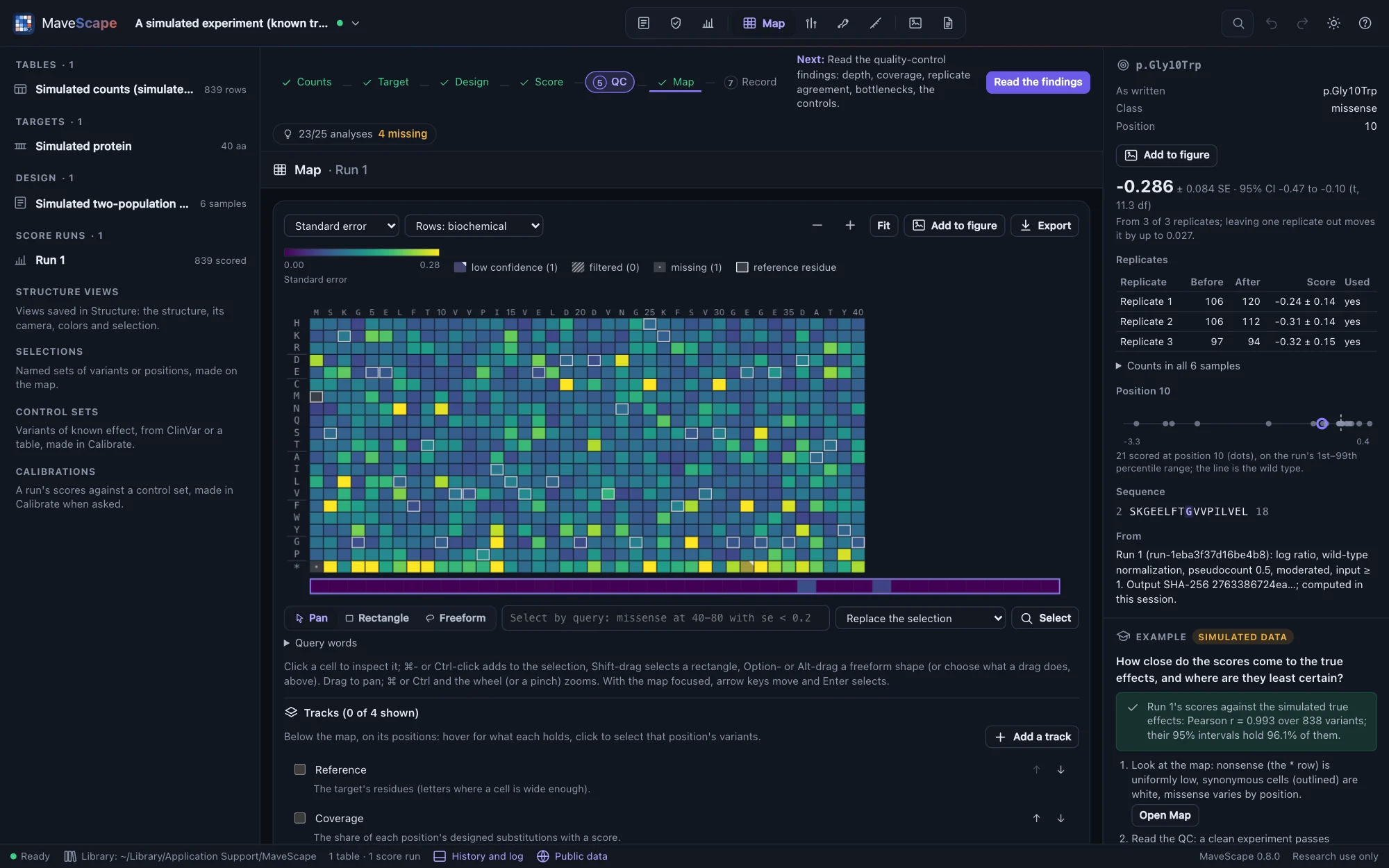
The map of the simulated example colored by standard error, with one variant's evidence in the inspector — The simulated example's map colored by standard error: the uncertain cells are the variants rare in the library.

The scores track the true effects closely: the guide shows the correlation (r = 0.99) once the run is scored, and how often the 95% intervals hold the true effects (96%; REML's would hold 93%).
The least certain scores are the variants with the fewest reads before selection.
Quality control passes: the counts vary as counting predicts.

A simulated time series (known truth)

A growth selection of a 40-residue protein in three replicates, sampled at five times over eight generations, simulated by MaveScape (seed 20261012) with every variant's true effect known. It opens scored by weighted regression on every time point.

The question: what does a regression on every time point add over the ratio of the first and last, and how linear are the time courses?

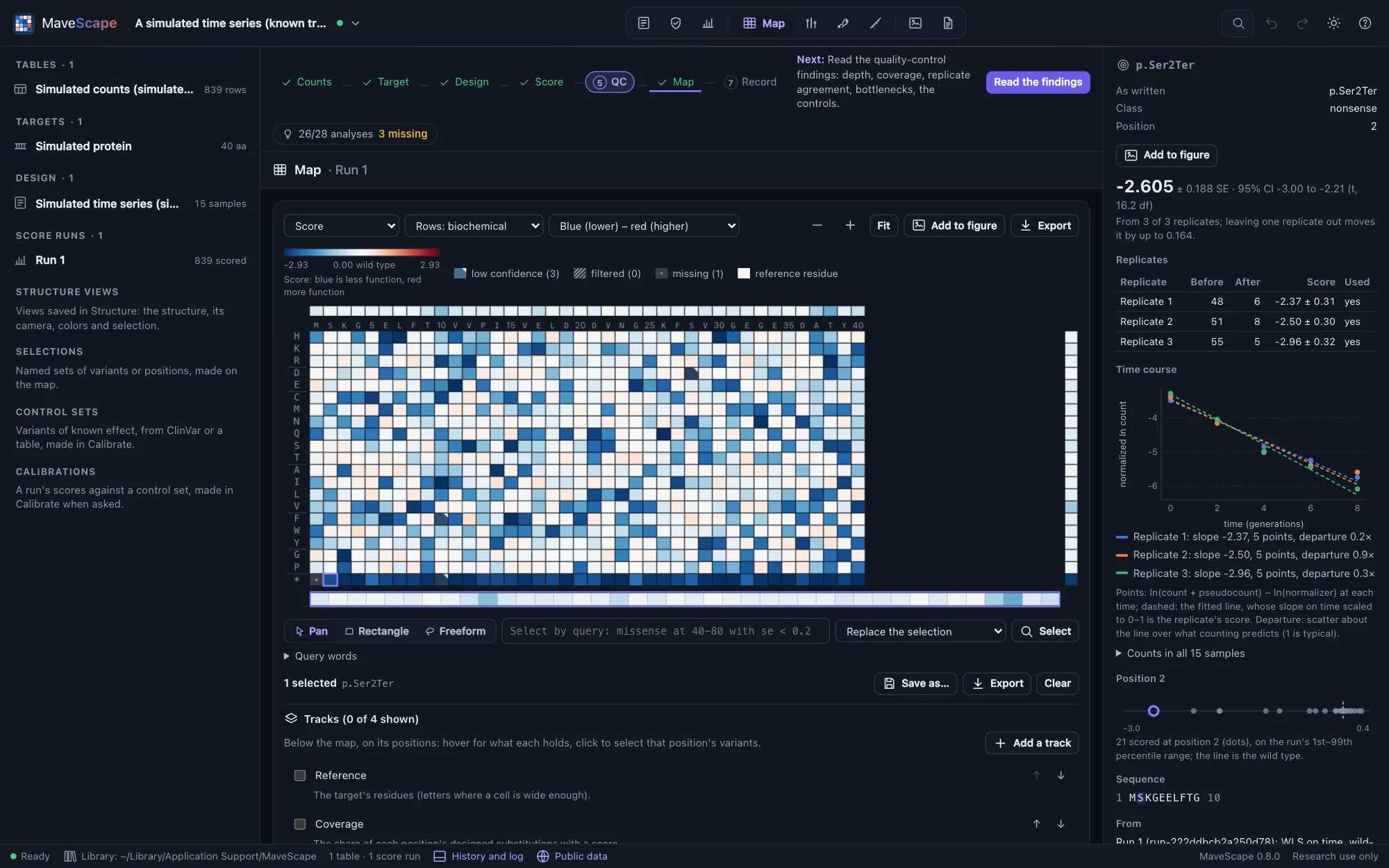
The map of the simulated time series with a nonsense variant selected and its time course in three replicates in the inspector — Click a cell: the inspector draws the variant's time course in each replicate, with the fitted lines.

The scores track the true effects (r = 0.99).
Quality control passes, including the two time-series findings: every fit uses every time point, and the time courses scatter about their lines as counting predicts.
Scored again by the log ratio of the first and last samples, the scores are a little noisier and their SEs larger: the middle time points carry information.
The times are in generations, so A score is the change per generation gives each score as a selection coefficient: the whole-course score over the eight generations.

A simulated sort-seq experiment (known truth)

Cells displaying every variant of a 40-residue protein sorted by a fluorescent reporter into four gated bins, in three replicates, simulated by MaveScape (seed 20261013) with each variant's true shift in log fluorescence known. The design records the gates and the cells sorted into each bin.

The question: how do the weighted average of the bins and the maximum-likelihood fit compare, and what limits the measurement: the cells or the reads?

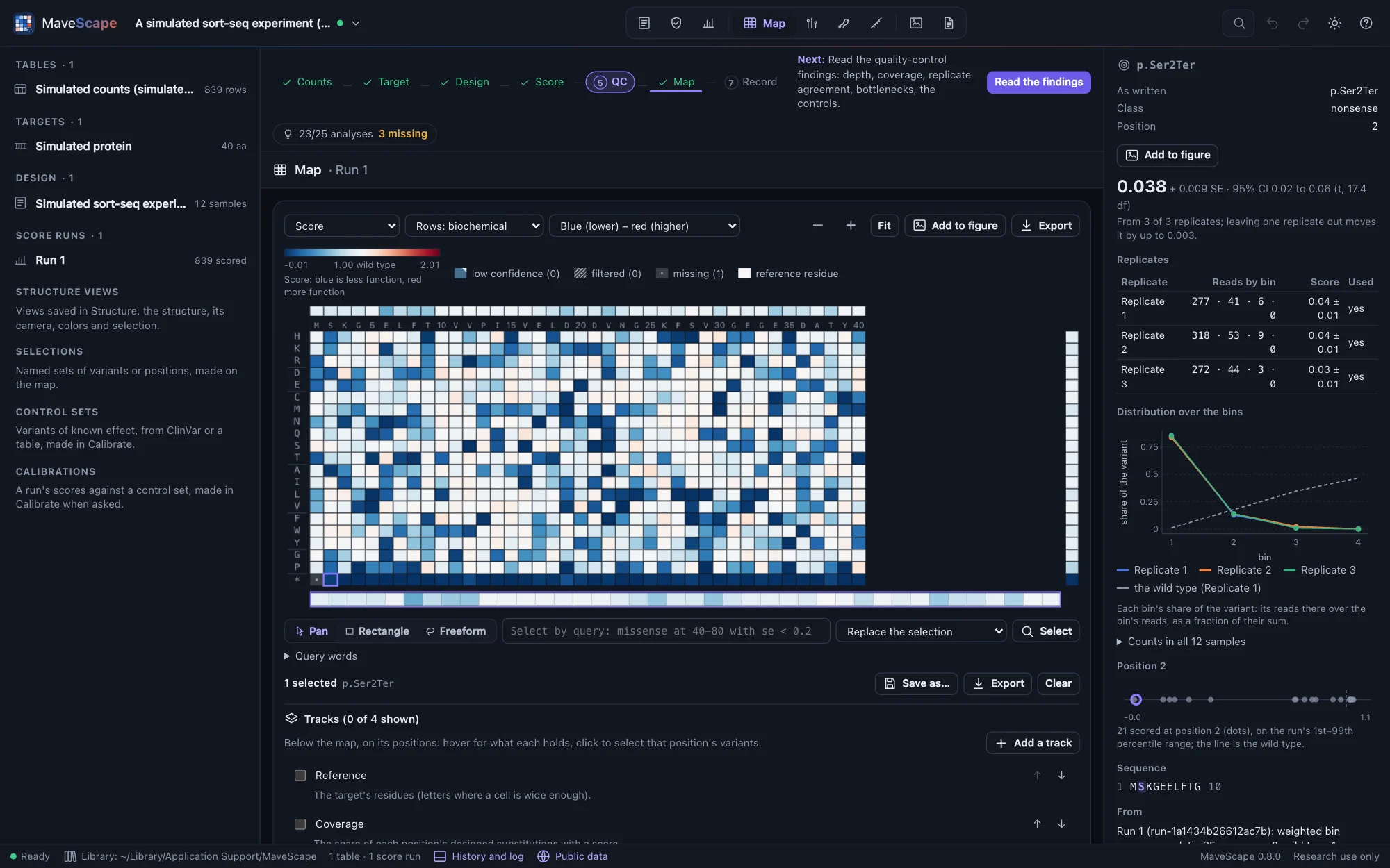
A nonsense variant's distribution over the four bins in each replicate beside the wild type's, in the inspector — Click a cell: the inspector shows the variant's distribution over the bins beside the wild type's.

Scored by the weighted average of the bins, scaled so that nonsense scores 0 and the wild type 1, the scores track the true shifts (r = 0.99).
Quality control reviews the variance beyond counting, about 2–3×: about 300 cells per variant were sorted against about 320 reads, so the cells, not the reads, limit what is known.
Scored by maximum likelihood, the scores follow the true shifts more closely, and their SEs account for the cells.

A simulated barcoded library (known truth)

Codon variants of a 30-codon gene in three independently made libraries, each variant carrying about five random barcodes, counted before and after selection, simulated by MaveScape (seed 20261014) with each variant's true effect known. The barcode-to-variant map misses 2% of the barcodes and gives another 2% two variants; 3% of the barcodes were made to be off from their variant by 1.5–3, as a barcode carrying a second mutation would be.

The question: do a variant's barcodes agree, which barcodes are outliers, and does scoring each barcode before combining them beat summing them?

The map names about 96% of the barcodes; those it gives two variants are left unmapped, and listed at import.
Quality control reviews the outlier barcodes, about 2% of those compared, and the variance between replicates beyond counting.
Summed per variant, the scores track the true effects with r = 0.985; each barcode scored and combined by REML, 0.996; summed with the outliers left out, 0.995.

A simulated two-condition experiment (known truth)

Every variant of a 40-residue protein selected from one input library under two conditions, without and with a ligand, in three replicates, simulated by MaveScape (seed 20261015). About 40 cells per variant were transformed and split between the two selections. Missense variants of a five-residue binding site (positions 12–16) lose about 1.5 in log fitness with the ligand only; every other variant behaves the same in both, so the true difference is known.

The question: which variants behave differently with the ligand, and how sure is each difference?

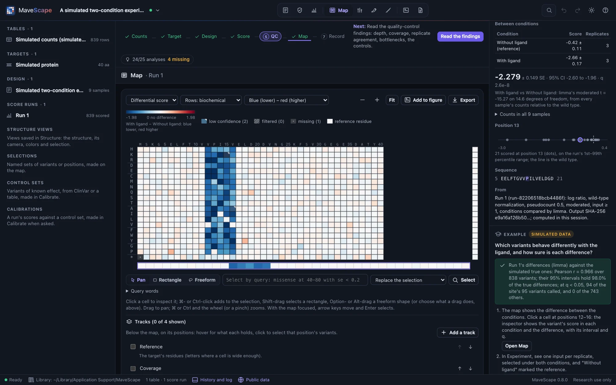
The map of the simulated two-condition example colored by the difference With ligand vs Without ligand, pale except a blue band at positions 12 to 16, with p.Pro13Ala in the inspector — The example opens on the map of the difference between the conditions; the binding site stands out.

The differences track the true ones (r = 0.97); limma's moderated t calls 94 of the site's 95 variants at q < 0.05, and none of the other 743.
Quality control reviews the variance beyond counting in each condition: about 40 cells per variant were transformed. Both conditions grew from the same cells, so the bottleneck cancels from their differences.
Compared as independent (Enrich2's z), the same differences have SEs about 1.6× larger: the input both conditions share is counted twice.

A simulated experiment with problems (known truth)

The two-population experiment again, with two problems planted: about 50 cells per variant carried into selection, recorded with each input, and a third replicate whose selection was far less even than the others' (seed 20261016). It opens in QC.

The question: can you find the two problems in the QC, and what do they do to the scores and their intervals?

The QC view of the simulated problems example: the variance beyond counting failing at 11.9 times counting, the agreement and an outlier replicate to review; the explanation says the recorded cells predict 2.5 times, more than they explain for replicate 3 — The variance beyond counting, read against the cells recorded: they explain replicates 1 and 2, not replicate 3.

QC fails the variance beyond counting and reviews the agreement and replicate 3, an outlier. The cells recorded account for the excess between replicates 1 and 2 (2.5× predicted, 2.2× seen); with replicate 3 the replicates differ about 12×.
From all three replicates the scores track the truth with r 0.96, and their 95% intervals hold 99.5% of the true effects: too wide, since the shared error model takes replicate 3's noise into every variant. DiMSum's terms, distorted by it too, put the excess after selection.
Remove replicate 3 in the Experiment view and score again: r 0.98, the intervals hold 96%, and DiMSum's terms put the bottleneck before selection, where it was planted. The guide shows both runs against the truth. Leaving a replicate out is a decision for the record: the history keeps it.

A simulated calibration with circular labels (known truth)

A noisy two-population selection of a 40-residue protein in three replicates (seed 20261017), and 100 classifications of its missense variants, each with the date it was last evaluated: 25 a side made before the assay was "published" in 2024, from the truth alone, and 25 a side made since, from the assay's own scores. The labels can be made a control set from the guide, or downloaded. It opens in Calibrate.

The question: half of the labels were made from the assay itself. Can you find them, and how far do they overstate the evidence its classes would give?

Of the 741 missense variants, 319 lose function in truth (a true effect of −0.4 or less). The control set of every label draws a warning: 50 were last evaluated since 2024 and may rest on the assay. Here they do, and 6 of them are wrong by the truth.
With every label, the abnormal-like class's OddsPath is 20.0, strong; the guide compares it with the truth at the same thresholds: a likelihood ratio of 11.2, moderate. With the labels made before 2024 (Last evaluated before 2024), 10.5 against a truth of 13.6.

Blank layouts

The start page also has three annotated files to fill in with your own data: a count table, a sample sheet and a target FASTA. FORMATS.md describes them and every other file MaveScape reads and writes.